Data cube measures

Data cube measures are numeric data values in Imply Polaris that are derived from your original table. For example, a measure can be an aggregation or a function output.

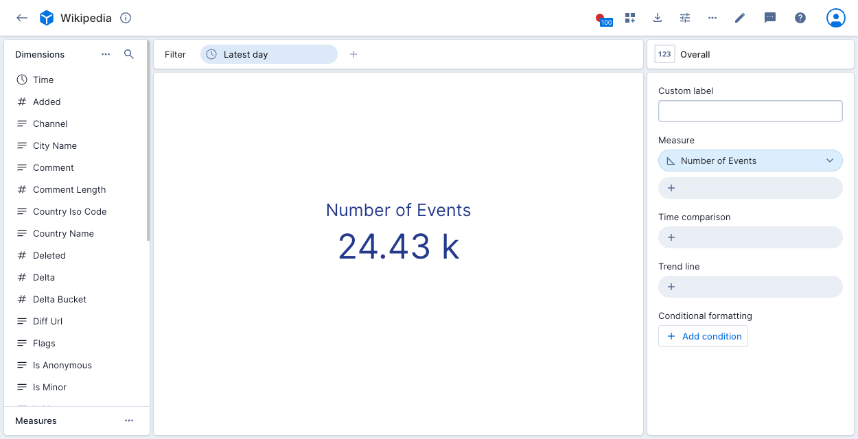
Polaris creates a measure that represents the event count by default if it's relevant to the data. For example, the Number of Events measure displays as follows:

Create a measure

To create a new measure, go into data cube edit mode and click the Measures tab.

Click the plus icon to create a measure and complete the following fields in the tabs, as outlined below.

General tab

• Name: Name of the measure.
• Description: Description of the measure to appear in the measure's Info pop-up window.
• Formula: Select one of the following:
  • Basic: A basic measure consists of a single aggregate function over a single column, with an optional filter.
    • Aggregate: Select the aggregate function.
    • Column: Select the column to aggregate.
    • Filter: Define and apply a filter.
  • Custom: A custom measure represents a post-aggregation transformation or computation. Enter a Druid SQL expression as the measure's formula. See Custom measure examples for more information.

Format tab

• Abbreviation: Select an abbrevation to apply to the measure format.
  Time format accepts formats supported by Moment.js. For example, YYYY/MM/DD HH:mm:ss displays time as 2023/10/18 15:36:40.
• Decimal places: Select the minimum and maximum decimal places to display.
• Comparison coloring: Select colors to differentiate comparisons.

Advanced tab

• Missing value fill: Choose how to fill missing values. See Measure fill options for more information.
• Scale behavior: Determines scale behavior in "continuous" visualizations such as the line chart. You can choose to always include zero for reference or not force zero into the scale.
• Transform: Transform the measure as a percentage of the parent segment or a percentage of the total.

When you've completed the configuration, click Save to save the measure.

Measure fill options

You can specify how to fill a measure on continuous visualizations, such as line charts.

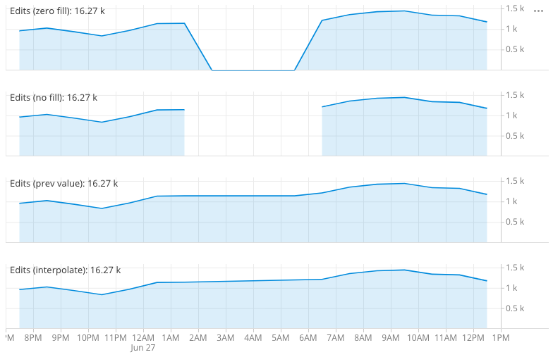
A data set can have gaps in data, for example, due to down time for the systems that generate the data. There are a few ways to handle the missing data in charts, as determined by fill options. The example shows four measures that are differentiated by differing fill options.

The possible options are:

• Zero filled (default): Fill missing data with zeros—most suitable if the measure represents an additive quantity.
• No fill: Leave missing data empty—suitable when missing values indicate that the data is not collected.
• Previous value: Fill missing data with last value seen—suitable for sensor type data.
• Interpolate values: Interpolate the missing data between the seen value—suitable for sensor type data.

Edit a measure

To edit a measure, go into data cube edit mode and click the Measures tab. Click the pencil icon next to a measure and update the measure properties as required.

Measure suggestions

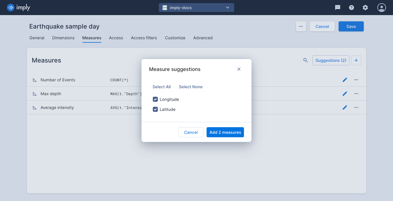
Click Suggestions at the top of the Measures page to review and add potential measures. Polaris scans the schema that underlies the dataset and automatically suggests measures with an appropriate aggregate for any columns not already represented.

You can use this feature if you add a new column to an existing table and want to include it in your data cube views.

Custom measure examples

This section describes some of the specific measure types. The sample expressions are in Pivot SQL format.

Filtered aggregations

Filtered aggregations are very powerful. For example, if your revenue in the US is a very important measure, you can express it as:

SUM(t.revenue) FILTER (WHERE t.country = 'United States')

It is also common to express a ratio of something filtered vs. unfiltered.

SUM(t.requests) FILTER (WHERE t.statusCode = 500) * 1.0 / SUM(t.requests)

Ratios

Ratios surface relationships in your data. Here's one that expresses the computation of CPM:

SUM(t.revenue) * 1.0 / SUM(t.impressions)

Quantiles

A quantile can be a very useful measure of your data. For large data sets it is often more informative to look at the 98th or 99th quantile of the data rather than the max, as it filters out corrupted values. Similarly, a median (or 50% quantile) can present different information than an average measure.

To add a quantile measure to your data, define a formula like so:

APPROX_QUANTILE_DS(t.revenue, 0.98)

It is possible to fine-tune the accuracy of the approximate quantiles as well as pick a different algorithm to use.

To learn more, see the Druid documentation.

Rates

In some cases, you may need to determine the rate of change (over time) of a measure.

There is a special function provided by Pivot PIVOT_TIME_IN_INTERVAL('SECOND') that gives the corresponding number of time units (first parameter) in the time interval over which the aggregation is running.

Therefore, it is possible to define a measure such as this one:

SUM(t.bytes) / PIVOT_TIME_IN_INTERVAL('SECOND')

This gives you the accurate rate of bytes per second regardless of your filter window or selected split (hour, minute, an so on).

Nested aggregation measures

You can define measures that perform a sub-split and a sub aggregation as part of their overall aggregation. This is required to express certain calculations which otherwise would not be possible.

The general form of the formula in a double-aggregated measure is:

PIVOT_NESTED_AGG(SUB_SPLIT_EXPRESSION, INNER_AGGREGATE(...) AS "V", OUTER_AGGREGATE("V"))

where:

• SUB_SPLIT_EXPRESSION is the expression on which the data for this measure is first split.
• INNER_AGGREGATE is the aggregate that is calculated for each bucket from the sub-split and is assigned the name V (which is arbitrary).
• OUTER_AGGREGATE is the aggregate that aggregates over the results of the inner aggregate, it uses the variable name declared above.

Examples of double-aggregated measures:

Netflow 95th percentile billing

When dealing with netflow data at an ISP level, one metric of interest is 5 minutely 95th percentile, which is used for burstable billing.

To add that as a measure (assuming there is a column called bytes which represents the bytes transferred during the interval), set the formula as follows:

PIVOT_NESTED_AGG(TIME_FLOOR(t.__time, 'PT5M'), SUM(t.bytes) * 8.0 / 300 AS "B", APPROX_QUANTILE_DS("B", 0.95))

Here the data is sub-split on 5 minute buckets (PT5M), then aggregated to calculate the bitrate (8 is the number of bits in a byte and 300 is the number of seconds in 5 minutes). Those inner 5 minute bitrates are then aggregated with the 95th percentile.

Average daily active users

When looking at users engaging with a website, service, or app, you might want to know the number of daily active users. You can calculate it as follows:

PIVOT_NESTED_AGG(TIME_FLOOR(t.__time, 'P1D'), COUNT(DISTINCT t."user") AS "U", AVG("U"))

Here the data is sub-split by day (P1D), and then an average is computed on top of that.

Switching metric columns

If you switch how you ingest your underlying metric and can't (or don't want to) recalculate all of the previous data, you can use a derived measure to seamlessly merge these two metrics in the UI.

Let's say you had a column called revenue_in_dollars, and for some reason you will now be ingesting it as revenue_in_cents.

Furthermore, right now your users are using the following measure:

SUM(t.revenue_in_dollars)

If your data had a "clean break" where all events have either revenue_in_dollars or revenue_in_cents with no overlap, you could use:

SUM(t.revenue_in_dollars) + SUM(t.revenue_in_cents) / 100

If instead there was a period where you were ingesting both metrics, then the above solution would double count that interval. You can splice these two metrics together at a specific time point.

Logically, you should be able to leverage Filtered aggregations to do:

SUM(t.revenue_in_dollars) FILTER (WHERE t.__time < TIMESTAMP '2016-04-04 00:00:00')
+ SUM(t.revenue_in_cents) FILTER (WHERE TIMESTAMP '2016-04-04 00:00:00' <= t.__time) / 100

Window functions

You can use window functions when defining a custom measure. For example, the following custom measure uses the RANK function:

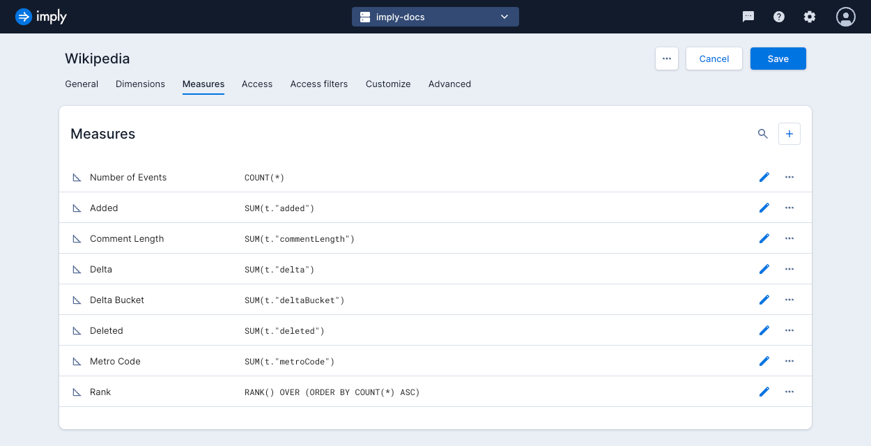
When applied to the Wikipedia data cube in the following example, the Rank measure assigns a rank to each channel, based on the channel's COUNT(*) value. A higher rank indicates a higher count:

Other custom measure examples

Here are more example expressions that you can use to build custom measures:

Counts all the rows in the data cube.

COUNT(*)

Counts the distinct values of the dimension.

COUNT(DISTINCT t."comment")

Counts how many rows match a condition. This example counts how many rows in the dimension are true.

SUM(CASE WHEN (t."dimension"='true') THEN 1 ELSE 0 END)

Returns the sum of all values for the dimension.

SUM(t."number_column")

Returns the smallest value of the dimension.

MIN(t."number_column")

Returns the largest value of the dimension.

MAX(t."number_column")

Returns the average value of the dimension.

AVG(t."number_column")

Returns the x quantile of the dimension. You cannot use a compound expression in this function.

APPROX_QUANTILE(t."dimension", 0.x)

Limits the number of records to apply a given aggregate. This example returns x or fewer results.

LIMIT (x)